In this post I explain how to derive vector data from Web Mapping Service (WMS) layers using QGIS.
These are notes on my workflow, not a full tutorial, and I've assumed some familiarity with the functions of QGIS. I am using QGIS version 3.18.
The input data is the Environment Agency's Risk of Flooding from Reservoirs outline maps. These maps are available to the public as three WMS layers: extent, depth, and speed. The layers are also presented via the EA's 'Check your long term flood risk' online service.
The three WMS layers are supplied under the terms of the Open Government Licence. However the underlying data, even in the simplified form depicted online, is not available for public access or re-use. The EA seems to think that disclosure of the vector data used to render the WMS layers would present a security risk.
This is one of the sticking points in my ongoing appeal to the Information Tribunal. The Environment Agency maintains that WMS is a "copy protected form" by means of which the outline maps have been published in a read-only format.
My own view is that releasing the underlying vector data is unlikely to make a material difference to the security risk, and that anyway a determined GIS user could vectorise comparable data from the WMS layers already available.
I demonstrate the second point in this post.
Vectorising a single location
We'll start with a basic example. First we load the WMS layer in the map canvas and navigate to our area of interest.
The images below show the maximum flood extent for Tortworth Lake, a privately-owned reservoir near Wotton-under-Edge in South Gloucestershire, at a scale of 1:5000.

As this is a WMS layer, we can overlay the outline on other data but we cannot manipulate the geographic features i.e. the extent polygon and the points and lines that make up the polygon.
Next we create a raster image of the polygon. We do this by adding the map (showing only the WMS layer) to a Print Layout and exporting the layout as a TIFF image (.tif or .tiff). QGIS will automatically georeference the TIFF file.
Close the print layout and load the TIFF file in the map canvas as a raster layer. The raster should look the same as the image served by the WMS. However raster data gives us access to raster bands: red, green, and blue expressed as values in a range from 0 and 255 for each pixel in the image.
Next we create a vector layer from the raster layer, using QGIS's Raster to Vector Tool. This tool calculates polygons by combining areas where neighbouring pixels have the same colour value in one of the raster bands.
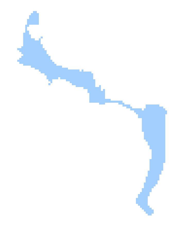
The first image below shows the vector layer created by the tool, and the second image shows the selected extent polygons after the polygon for the background area outside the extents has been deleted.
We can now save the vector layer in a file format such as shapefile or GeoPackage. This vector data can be used without a connection to the WMS.


Producing vector files from the WMS layers for the maximum flood depth and speed (shown below) is a little more complicated, because we also need to attribute the polygons with the depth and speed bands represented by the colour values in the raster bands.


Semi-automated vectorisation using Atlas functions
Vectorising the outline flood maps for a small geographic area is only a few minutes' work in QGIS. But is it practical to vectorise the same WMS layers across all of England?
That will require us to export tens of thousands of TIFF files, then stitch them together before converting their raster values to polygons. Lots of work.
Fortunately QGIS's print composer has atlas functions that enable us to zoom from location to location and export a TIFF file for each location automatically.
First we have to create a coverage layer so that QGIS knows which locations to capture. In this case I created a coverage layer using Ordnance Survey's National Grid at a resolution of 1 km.
I removed all the grid squares that did not overlap with any reservoir flood extents. This was a manual process and took a tedious amount of time because it involved scrolling across the whole of the extent layer at a scale of 1:40000. You can download the output (0.7 MB) as a shapefile.


Creating the TIFF outputs involved a lot of trial and error with the layout settings. I ended up rendering an image of 3000 x 3000 pixels for each grid square, but that may be unnecessarily large. Part of the problem was that the outline maps served by the WMS are not simplified to a common resolution.
The next step is to stitch a batch of our TIFF files together using QGIS's Build Virtual Raster plugin. A virtual raster is a special type of raster layer that presents a directory of raster images as if they were a single seamless layer.
The following image shows the combined raster data for the SK area of the National Grid, which includes Sheffield and Nottingham.

We can create vector files from the virtual raster layer in the same way as from a normal raster layer, using QGIS's Raster to Vector Tool.
As a proof of concept I have produced vector files for Risk of Flooding from Reservoirs outline maps covering the SK area (extent, depth and speed) and made them available in GeoPackage format as an open data download (26.2 MB).
Information warning
In principle the above workflow should provide new vector data that is functionally equivalent to the original vector data used to render the WMS layers from which the new vector data is derived.
For the purposes of developing this workflow, I have not done any quality assurance on the outputs.
Spot-checking indicates the outputs are visually identical to the WMS inputs at small scales. However there is no way to accurately measure congruity without access to the underlying data.
Technically (and legally) the vector outputs are not the same information as the vector data underlying the WMS inputs. The outputs lack the authority that a direct release of outline maps in vector format by the Environment Agency would have.
Attributions for data used to produce images in this post:
Contains OS data © Crown copyright and database right 2021.
© Environment Agency copyright and/or database right 2019. All rights reserved.
Aerial imagery © Google.
")
Image credit: Tortworth Lake, South Gloucestershire by kennysarmy (CC BY-NC-ND 2.0)